Monte Carlo method for Pi
The Monte Carlo methods are a class of algorithms that rely on repeated random sampling to calculate the result. These methods are used in Engineering, Statistics, Finance and many other fields.
Our objective is to familiarize ourselves with a Monte Carlo method for
computing the Pi (π) number. First, we will implement a
sequential version of the method. And then, we will use OpenMP to parallelize
the sequential version.
Computation of Pi
If you don’t know what π is, it is that number which has
something to do with circles. More precisely, the area of the disk with the
radius r is equal to π * r^2.

If the radius of the circle is equal to one, then the area of the disk is equal
to π.
Further, let’s inscribe a circle in a square. If the length of the side of the square is equal to two, then the radius of the inscribed circle is equal to one.
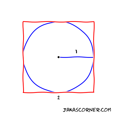
Now, we divide the area of the circle with the area of the square

If we multiply this fraction by four, we get the value of π.
A simple way to compute the fraction is to generate the points in the square and count the number of points which lie in the inside of the circle.
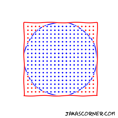
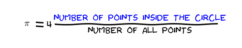
The approximation of the π is
Monte Carlo method for Pi
The Monte Carlo method uses the previous idea to compute the value of
π. The method randomly generates points in the square
[-1, 1] x [-1, 1] and counts the number of points in the
inside of the unit circle. The result is four times the fraction between the
number of points which lie in the inside of the circle and the number of all
generated points.
Implementation
Uniform points
The first step of the implementation is to uniformly generate random points.
The <random>
standard library is appropriate for such a task. In order to generate random
points with the library, we need to specify two things:
- the generator, which generates the uniformly distributed numbers and
- the distribution, which transforms the numbers from the generator into the numbers that follow a specific random distribution.
We use
std::default_random_engine
as the generator and
std::uniform_real_distribution<double>
as the distribution. We initialize the internal state of the
generator with the std::default_random_engine::seed member
function. Finally, we generate an uniform random sample (x,
y) in [-1, 1] x [-1, 1].
std::default_random_engine generator;
auto seed = std::chrono::system_clock::now().time_since_epoch().count();
generator.seed(seed);
std::uniform_real_distribution<double> distribution(-1.0, 1.0);

double x = distribution(generator);
double y = distribution(generator);
We encapsulate the random generation of the points in the class
UniformDistribution. The constructor takes care for the
initialization of the generator and the distribution. The member function
UniformDistribution::sample generates a random sample in the
interval [-1, 1]. The following code is then equivalent to
the code above.
UniformDistribution distribution;

auto x = distribution.sample();
auto y = distribution.sample();
The source code of the UniformDistribution is available
here.
Monte Carlo method
The next function describes the Monte Carlo algorithm for π.
double approximatePi(const int numSamples)
{
    UniformDistribution distribution;

    int counter = 0;
    for (int s = 0; s != numSamples; s++)
    {
        auto x = distribution.sample();
        auto y = distribution.sample();

        if (x * x + y * y < 1)
        {
            counter++;
        }
    }

    return 4.0 * counter / numSamples;
}
The input of the function is the number of samples. The function generates
samples (x, y) in [-1, 1] x [-1, 1] and
counts all the samples which lie in the inside of the circle with radius
one. The approximation of the π is four times the fraction
between the number of samples, which lie in the inside of the circle, and the
total number of samples. This approximation formula for the value of
π was derived above.
Examples
The quality of the result depends on the total number of samples. The higher number of samples increases the accuracy of the solution. The next output illustrates this phenomenon.
$ ./monteCarloPi
real Pi: 3.141592653589...
----------------------------------------
approx.: 3.2              (10 samples)
approx.: 3.28             (100 samples)
approx.: 3.128            (1000 samples)
approx.: 3.1668           (10000 samples)
approx.: 3.14632          (100000 samples)
approx.: 3.140976         (1000000 samples)
approx.: 3.1421832        (10000000 samples)
approx.: 3.14189536       (100000000 samples)
approx.: 3.14159724       (1000000000 samples)
----------------------------------------
real Pi: 3.141592653589...
We can see that the results are more accurate with higher number of samples. Another observation is that the Monte Carlo method is an approximation algorithm – it returns an approximation of the result not the exact solution.
Since the algorithm depends on the random sapling, two executions of the same program give different results.
A valid concern is whether the Monte Carlo methods are useful at all. Why would
someone use the method which returns approximate results (and these results
might vary from one execution to the other)? Of course the Monte Carlo method
for π is not very useful, because the value of
π is very well known.
But there exist problems for which it is impossible to compute results in a reasonable time. Here, the Monte Carlo methods are useful, because they can provide an approximation of the result within an acceptable time. Sometimes, it is better to have an approximation of the result than no result.
Since the Monte Carlo methods depend on a repeated independent random sampling, they are especially appropriate for parallel execution. Each thread can independently compute many samples.
In the next article, we will parallelize the Monte Carlo method for
π with the help of OpenMP.
Summary
In this article, we learned a Monte Carlo method for the approximation of
π.
Links